In the previous blog, Power Query Part 1, we focused on the E and the L of ETL in Power Query. As promised, in this blog, we will shift our focus to look at the Transform step.

There is a whole raft of transform and cleaning commands in Power Query. Suffice to say, we won't be able to have a look at all. Instead, let us look at a few common commands with the aid of the Sample Art Store data I've mocked up.

I'm sharing the Sample Art Store data so you can follow along. There is a quote I came across, and it's very fitting to share here: "Tell Me, I'll Forget; Show Me, I'll Remember; Let Me Do it, I'll Understand". So, what are you waiting for? Download the sample data and follow me~

Before we commence, let's look at the data and the list of Power Query Commands we will walk through together:

Sample Art Store Data

There are two tabs: Inventory and Customer Purchase. We will be combining the tables in Power Query.

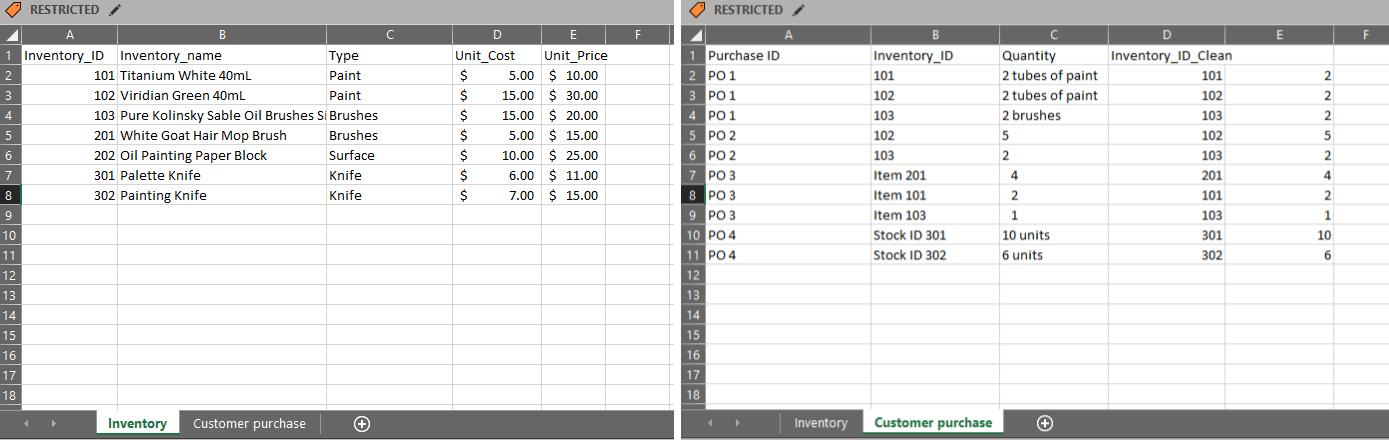
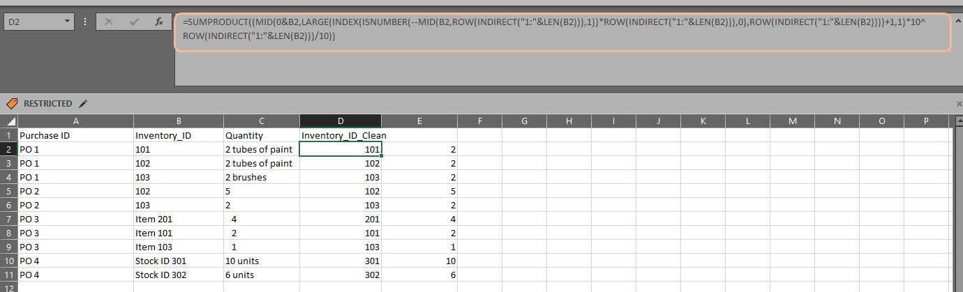
In the Customer Purchase table, you'll notice that the two last columns contain data that's the same as Inventory_ID and Quantity. When you download the Excel file, take a closer look at the formula required to extract the numerical values. It's overwhelming and horrible! But not to fear, extracting the values we want using Power Query is a walk in the park.

Power Query Commands List

These are the six commands we will be examining:

1. Split Column
2. Trim
3. Extract
4. Sort
5. Merging queries
6. Conditional Column

Load the Data

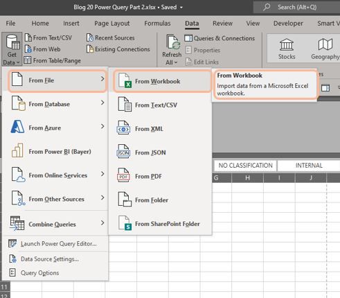
First, open Excel and pull the Sample Art Store data into the Power Query Editor. Navigate to the Data tab on the ribbon and move to the Get & Transform group to import the data source.

So, it’s: Data> Get & Transform Data > Get Data > From File > From Workbook > Sample Art Store.xlsx

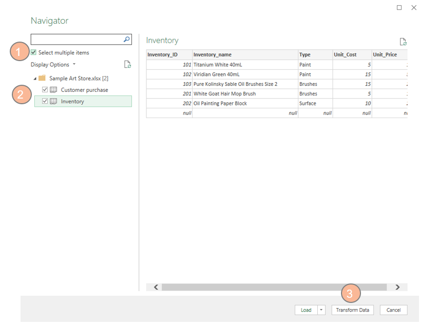
Once the Sample Art Store excel workbook is selected, it will open the Navigator window.

In the Navigator window, you'll see two tables. Now, please do the following:

1. Tick Select multiple items
2. Tick Customer purchase and tick Inventory
3. Click Transform Data

Once you've clicked on Transform Data, you'll be taken to the Power Query Editor- this is where the fun begins!

Split Column

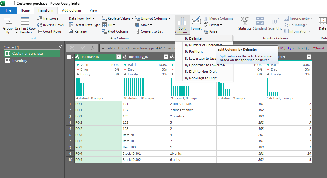
We will start with the Customer purchase table. In the first task, we want to clean the Purchase ID column. The text PO preceding the number is not required, so let's remove it using Split Column.
Do the following steps:

1. Select the Purchase ID column
2. Navigate to the Transform tab.
3. Locate Text to Column group,
4. Click Split Column, then By Delimiter.
5. In the Split Column by Delimiter window, choose Space from the Select or enter delimiter box.
6. Choose Each occurrence of the delimiter.
7. Click Ok

Note the above are default selections.

You'll now see two columns labelled Purchase ID.1 and Purchase ID2.

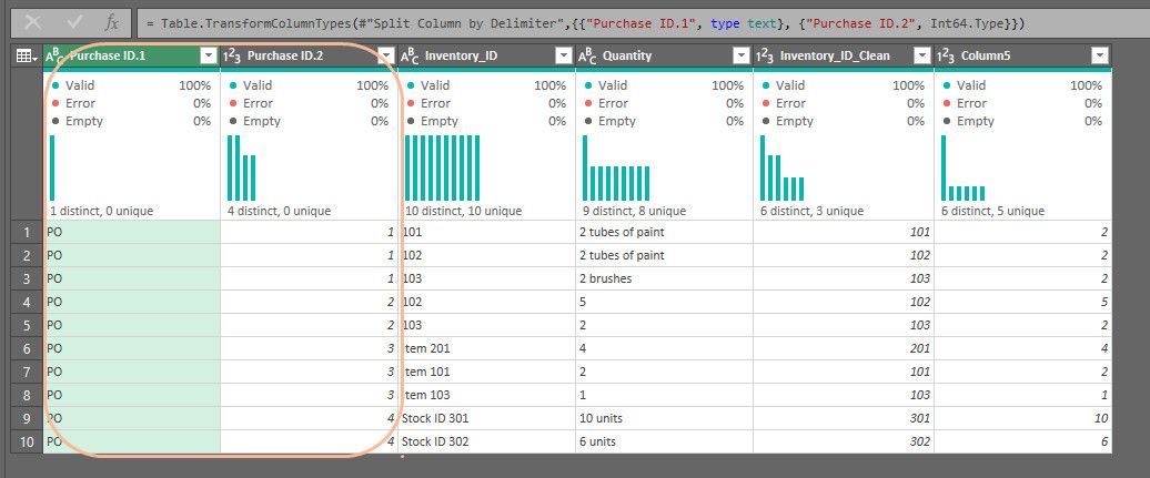
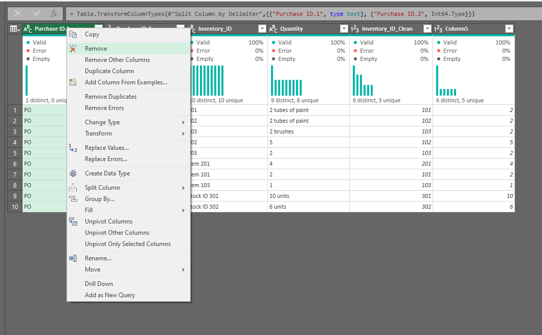
We don't need Purchase ID.1, so let's eliminate it by right-clicking the column and selecting Remove.

Let's also edit the label for Purchase ID.2 to Purchase ID by double-clicking on the column heading.

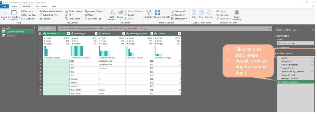
I'll like to draw your attention to the APPLIED STEPs box of the Power Query Editor. Power Query records each step for you as you change the data. This feature is useful when you have to repeat the same cleaning steps when you get new files.

If you make a mistake and want to undo it, click on the x to delete. You can also rename the steps as well. I like to rename the steps, so it's more descriptive. It helps with debugging.

Trim

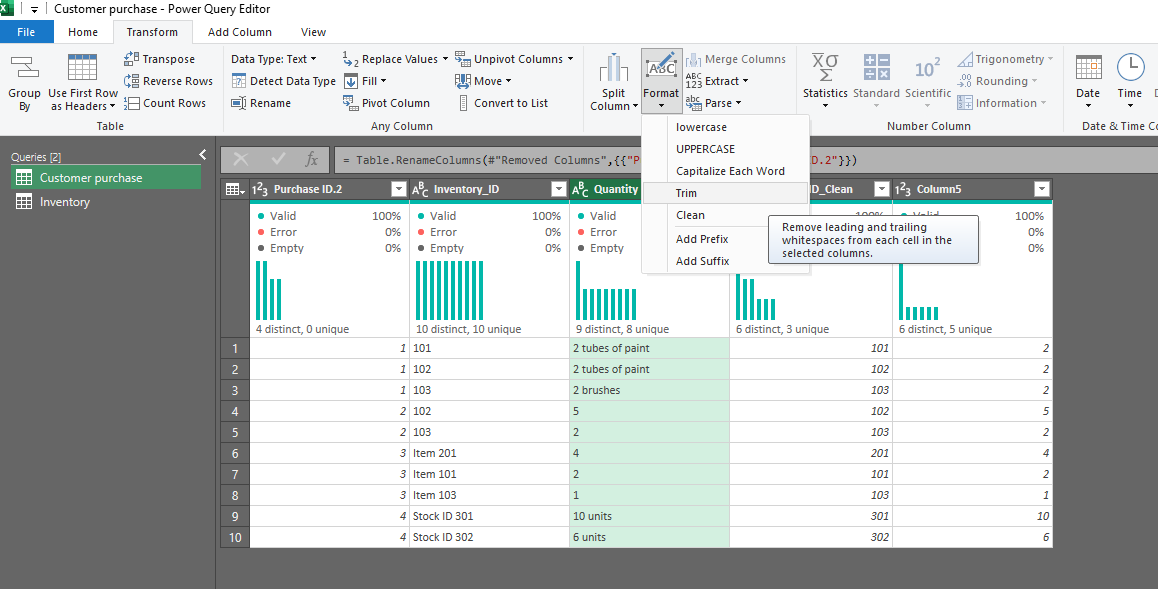
Next, we're going to work on the Quantity column. It may not be apparent, but there are a couple of leading spaces in the quantity column. So let's Trim away these annoying spaces.

1. Select Quantity column
2. Navigate to the Transform tab
3. Go to Text To Column group
4. Click Format, then Trim

Extract

Continuing the Quantity column. We don't want the descriptive text following the quantity, so we will remove all the text. Like Split column, lets do the following:

1. Select Quantity column
2. Navigate to the Transform tab.
3. Locate Text to Column group,
4. Click Extract, then Text Before Delimiter.
5. In the Text Before Delimiter window, enter a Space.
6. Click Ok

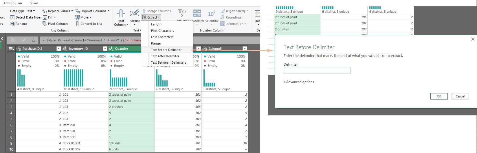
Now, all the text has disappeared, leaving behind numerical values only.

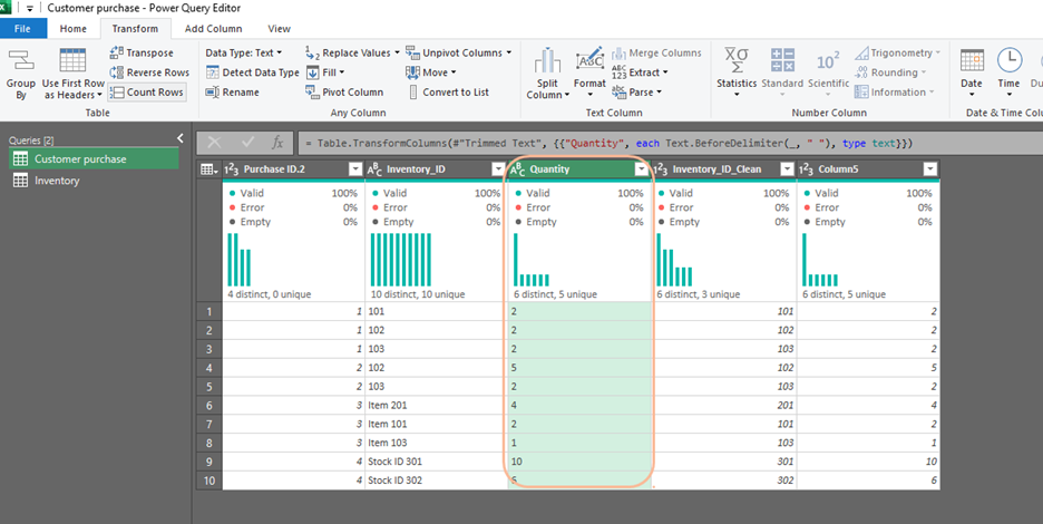
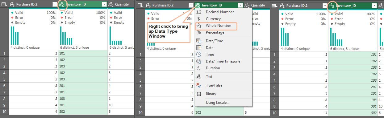
Ok, we're going to do another Extract. This time we will apply to the Inventory_ID column. Again, we want the numerical numbers and not the text. You might have noticed in the above screenshot that there is an Extract option for Last Characters. That's what we are going to use here. But before we do that, there are a few leading and trailing spaces, so let's apply Trim to the column first. Once that's done, let's extract. so,

1. Select the Inventory_ID column
2. Go to the Text Column grouping in the Transform tab
3. Click Extract, then Click Last Characters.
4. In the Extract Last Characters window, type 3 in the Count box
5. Click ok

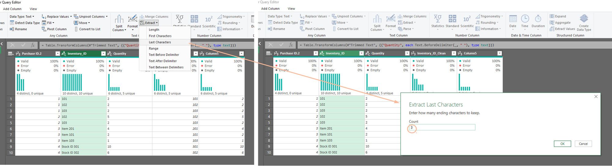
This is what it should look like after you've gotten rid of the text.
However, noticed the data type? It's text, not integer (or whole number, as called in Power Query). We need to change it to integer so we can later merge it with the Inventory table. Power Query won't allow you to combine the column if the column you are joining has different data types.

Sort

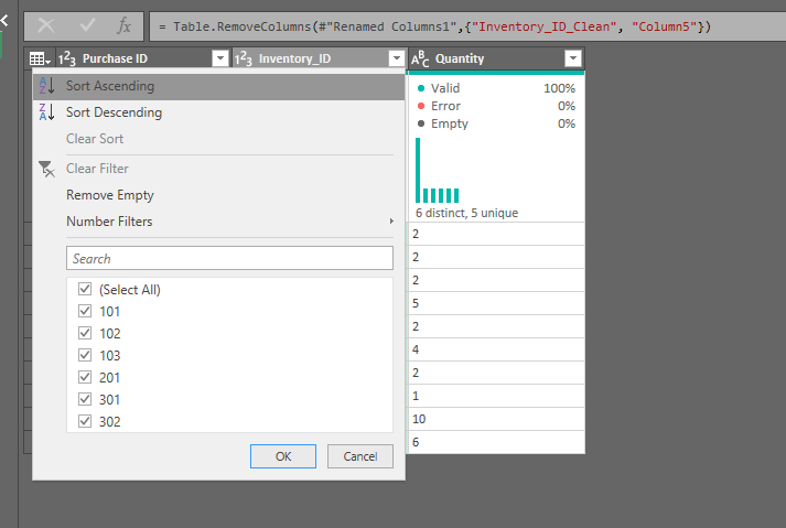
All of the data in the Customer Purchase table is now clean. Let's quickly remove the last two columns in the table as they duplicate Inventory ID and Quantity. To do so, click one column, hold down CLT key, click the second column, right-click, and then click Remove Columns.

Let's then sort Inventory_ID, so it's in order. Click on the Inventory_ID heading and then click Sort Ascending, followed by Ok.

Merge Queries

When we're preparing data, it's pretty often that we want to merge tables (commonly referred to as joining tables). I won't describe and explain the types of joins here. It's a big topic, so I will leave it for another day.
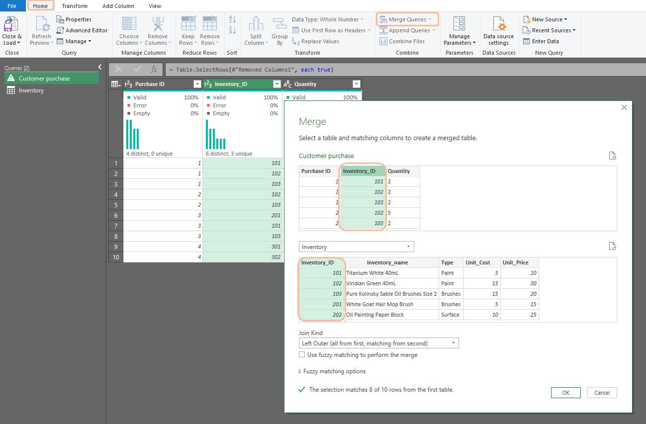
Let's join the Customer Purchase table with the Inventory table. With the Customer Purchase sheet selected on the far-left side of the Power Query editor,

1. Navigate to the Home tab
2. Click Merge Queries from the Combine group. This will bring up the Merge window. The Customer purchase table will appear on top. Directly below that is a drop-down box where you can choose another table. Let's select the Inventory table.
3. We need to specify which column to join the two tables on. The common column between the two tables is the Iventory_ID, so let's select the column from both tables.
4. In terms of which type of join, left it as default: Left Outer (all from first, matching from second).
5. Click Ok.

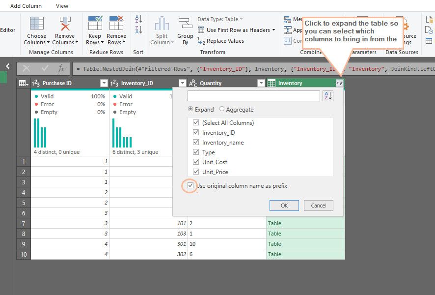
You'll see a new column in the Customer purchase table from within the Power Query Editor. We need to expand the contents of that new column. Click the Expand button in the new column's header, and a window will open.

By default, all the columns from the Inventory table will be added, but you can choose which column you want to bring in by Unselecting the ones you don't want.

Before you Click Ok, uncheck the box that says "Use original column name as prefix" unless that's what you want.

Your table should look like this:

Conditional Column

Notice that the table has a Unit_Cost and Unit_Price column. Let's create two new columns: Total_Cost and Total_Price, out of the two columns by multiplying each with the Quantity column. Before we do this, let's change the data type for Quantity from Text to Whole Number. It will throw an error if we don't do that first. After that's done,

1. Go to Add Column on the Ribbon
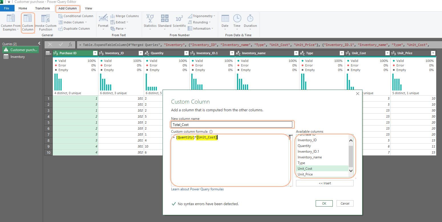
2. Click Custom Column from the General group. This will bring up the Custom Column window.
3. Under the Custom Column window, type " Total_Cost" under the New column name
4. Move to the box under the Custom Column formula.
5. Place your cursor after the = sign shown. Double-click Quantity from the Available columns box on the far-right side of the window, type * (mean multiply) and then double-click Unit_Cost from the Available columns box.
6. Click OK

We have to repeat steps 1 to 6 to create the Total_Price column, but remember to replace Unit_Cost with Unit_Price in the formula box.

Right, now, the dataset is ready. Now we can load this to an Excel table. Check out Power Query Part 1 if you aren't sure how to load it.

Once you become fluent with Power Query, a data set like this should take you no more than a few minutes.

I hope you enjoyed this blog. There are heaps more commands that I think you add to your arsenal. Here are a few more common ones that I recommend you look into:

• Remove Duplicate
• Conditional Column
• Append Queries
• Transpose
• Unpivot
• Fill down
• Replace Values